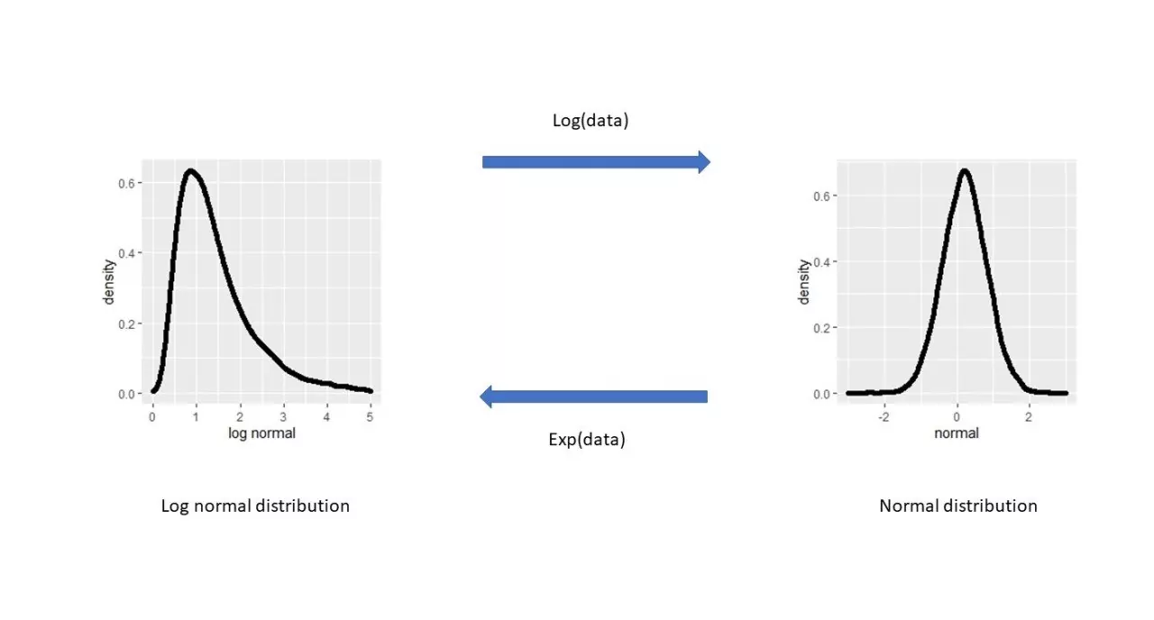
Log or not log (transform data) that’s the question
By Jean-François Michiels (Senior Manager Statistics and Data Science at Pharmalex), Deniz Akinc (Manager Statistics and Data Science at Pharmalex) and Marieke Verweij (Scientist at Janssen)
In the analysis of (bioassay) data, there are assumptions to be validated such as data is expected to be approximately normally distributed with a constant variance across the specified range. Most of the time, the constant variance (homoscedasticity) assumption cannot be satisfied in bioassay data. In case this assumption fails, the estimate of within-assay variance will be unreliable, which will also affect the computation of the overall percent coefficient of variation (%CV). Log transformation is the most common used tool to satisfy these assumptions of the analysis, specifically the constant variance assumption.
The focus of this article is to demonstrate how the %CV computation changes when performing an analysis with log-transformed data instead of untransformed data. The following example is used to illustrate this effect of log-transformation and how to use JMP to correctly calculate the %CV of transformed data.
Illustration by cell measurements analysis
A concentrated cell suspension is prepared using the manual counting as the reference. This concentrated cell suspension is then diluted to prepare two additional cell concentration levels. Using the technique to be evaluated, each cell level is measured three times. The whole experiment is repeated on four different days (aka runs).
The data structure is shown below.
Table 1. The structure of the data
In order to compute the %CV, the following linear mixed model is fitted to the data;
where
- Y are the measured and theoretical cell concentration
and
are the intercept and slope of the model, respectively
is the random run effect
is the residual error
From Figure 1, it can be observed that the residuals computed from different cell concentration levels do not have the same variability (i.e. heteroscedasticity).
Figure 1. The plot of predicted values versus residuals with untransformed data.
When the following linear mixed model is fitted to the log-transformed data;
the residuals have roughly the same variability across the different cell concentration levels, see Figure 2. Some difference in variability between levels can be observed. Nevertheless, those differences are less extreme than the model without log-transformation.
Figure 2. The plot of predicted values versus residuals with log-transformed data.
The second model is preferred because the log transformation of the response (measured cell concentration) corrects the heteroscedasticity of the residuals and the log transformation of the explanatory variable (theoretical cell concentration) is required to obtain a linear trend.
Coefficient of variation after log transformation
The %CV is a unit-less measure of variation. Under normal distribution, it was defined as;
where
is the standard deviation
is the mean
When data were applied a log-transformation, another formula is required to obtain the %CV in the original units. The formula below is provided for a natural-log transformation:
where
- e is exponent
- Log is natural-base log (ln)
is the standard deviation
The formula below is provided for 10 base-log transformation. The two expressions are mathematically equivalent.
If the formula for normal distribution is used instead of the formula for log-transformed data, an incorrect %CV will be obtained.
In addition, the correct formula should be carefully applied as it is prone to errors (such as, use of variance instead of standard deviation or, if the formula for natural-log transformation is used although the data has been log 10-transformed).
Implementation of the formula in JMP
JMP is a statistical software, widely used for its user-friendly interface. In addition, the JMP scripting language allows the creation of add-ins.
By using the “Fit Model” menu in JMP (see in Figure 3), the second model (above) is fitted. Note that the model is fitted by making the log 10 transformation in the data table and not by using the utility in the model dialog.
Figure 3. The screenshot of the “Fit Model” menu in JMP.
The variance components are obtained in Table 2 given in a newly opened result screen. These results can be extracted to a JMP data table by right-clicking on this table.
Table 2. The estimates of Variance components obtained by the second model with log-transformed data.
To compute %CV, one can enter the formula editor and create the above-mentioned formula.
Alternatively, a JMP add-in, as shown in Figure 4, has been implemented to add the formula of %CV in the formula editor. This add-in can be freely downloaded here (bottom of the page).
https://www.pharmalex.com/our-services/custom-software-development/
After downloading the add-in, one can install it by double-clicking on it and click on the menu “Add-Ins” and “Install CV formulas in the formula editor”. This latest step needs to be repeated for each JMP session.
When editing the formula to obtain the %CV, the formulas are available in the formula editor in a new category named “Pct CV from mixed models”. Formulas are provided for natural log and log 10; and using variance and standard deviation. In addition, in the scripting editor, the description and one example are provided for each of the formula (Figure 4).
Figure 4. The screenshot of %CV computation add-in in JMP.
And if we compute the %CV per concentration level
In the scope of assay validation, %CV is usually provided per concentration level. Using the same tools, the overall %CV can be compared to the %CV per concentration level (Table 3). It can be observed that the %CV are quite different between cell concentration levels, as already noted in the residual plot. if the acceptance criteria were set at %CV < 20% for repeatability and intermediate precision, either per concentration level or in total, the validation of the method would have succeeded.
Table 3. The %CV per concentration level and overall with log-transformed data. In the assay validation terminology, Run, Residual and Total corresponds respectively to between-run, repeatability and intermediate precision.
Conclusions
We have shown that log-transformation is extremely useful for correcting heterogeneity of variances of residuals. Although the %CV under log transformation is not complex, it is easy to make errors, while implementing the formulas. The implementation of the formula in JMP makes the computation of errors less prone to errors. This example demonstrated that JMP is much more than a click-button software, the possibility of scripting analysis is highly valuable.Contact us now


